Accessibility:
minutes of walking, not kilometres

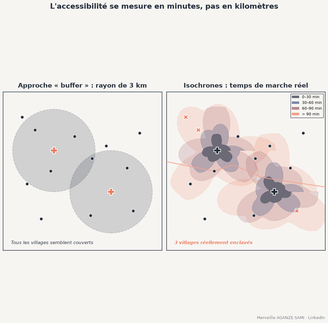
Assessing the geographic coverage of a service frequently relies on a fixed radius drawn around each facility: five kilometres for a health centre, an hour's walk estimated as a flat rate. Settlements inside are counted as served.

This approach has an immediate limitation. A radius assumes straight-line movement at constant speed, an assumption rarely met in rural settings: marked relief, a watercourse with no crossing point or a track impassable in the rainy season lengthen the actual journey considerably. Coverage computed this way is systematically overstated, and the error concentrates precisely on the hardest-to-reach areas.

1. Two families of method

The first computes travel time along a network of roads and paths, each segment assigned a speed according to its type and condition. This approach suits situations where the network is well documented and where movement actually follows it.

The second builds a cost surface on a grid: each cell is assigned a travel speed based on land cover, slope and the presence of a route, then an algorithm computes minimum cumulative time from each service point. This approach accommodates off-network movement, which is common in rural areas. Comparison of the two families shows that the choice appreciably affects results and must be justified (Delamater et al., 2012).

2. The parameters that determine the result

• Speeds by surface type. Paved road, track, footpath, savanna, dense forest, marshland: the values adopted are the model's heaviest assumption. They are best calibrated against actually observed journey times rather than taken from a publication.
• Mode of travel. Walking, motorcycle, vehicle, or a combination. A single model applied to the whole population conceals considerable differences in access between households.
• Season. In tropical settings, passability varies strongly between dry and rainy seasons. Two sets of isochrones are more informative than one, and the gap between them is itself a vulnerability indicator.
• Crossings. Bridges, ferries and fords condition access in a binary way. Omitting them from the data produces results that are wrong, not merely imprecise.
• Point of origin. Settlement centroid, mapped buildings or a population grid: the choice changes computed times, especially for extended settlements.

3. Travel time is not enough

A useful distinction separates physical access — reaching the facility — from effective access — receiving a service there. A facility reachable in thirty minutes but without staff, or saturated, does not provide the access the map suggests.

So-called floating catchment area measures incorporate this dimension by relating potential demand to available capacity within a given time radius (Luo & Wang, 2003). They produce an accessibility indicator closer to lived reality, at the cost of additional data on facility capacity.

4. Available data and their limits

Friction surfaces and global travel-time maps are now available and provide a useful starting point where local data are lacking (Weiss et al., 2018) (Weiss et al., 2020). Their resolution and the generality of their assumptions nonetheless make them a complement rather than a substitute for local modelling where the decision concerns siting a facility.

• Network completeness. Collaborative databases cover rural areas unevenly. A track missing from the database produces an artificially cut-off area; a non-existent path produces the reverse. Verification against recent imagery is necessary before any computation.
• Terrain model resolution. Coarse resolution smooths slope breaks and understates times in rugged terrain.
• Field validation. A handful of journey times reported by residents, compared with computed values, is enough to detect a major parameterisation error. This check is inexpensive and rarely performed.
• Reading the thresholds. The time classes adopted — thirty, sixty, ninety minutes — steer the conclusion. They must correspond to documented operational thresholds, not to an aesthetic gradation.

5. What this changes for targeting

Moving from a radius to a travel time generally changes the list of settlements considered unserved, and the difference concentrates in areas of marked relief or cut off by a watercourse. These are precisely the areas where intervention is most warranted and where the theoretical radius led to concluding that coverage was sufficient.

The resulting indicator — the share of the population more than a given walking time from a facility — also has the advantage of being directly interpretable by a partner, which a straight-line distance is not.

Accessibility is measured in travel time, not in straight-line distance. A map that conflates the two overstates coverage precisely where access difficulties are greatest.

Merveille Aganze Sami

MEL & Database Management Advisor. 9+ years of experience in monitoring & evaluation, GIS and digitalization with international organizations (GIZ, Enabel) in DR Congo.

LinkedIn Contact me

References

- Delamater, P. L., Messina, J. P., Shortridge, A. M., & Grady, S. C. (2012). Measuring geographic access to health care: raster and network-based methods. International Journal of Health Geographics, 11, 15. doi.org/10.1186/1476-072X-11-15
- Luo, W., & Wang, F. (2003). Measures of Spatial Accessibility to Health Care in a GIS Environment: Synthesis and a Case Study in the Chicago Region. Environment and Planning B: Planning and Design, 30(6), 865–884. doi.org/10.1068/b29120
- Ray, N., & Ebener, S. (2008). AccessMod 3.0: computing geographic coverage and accessibility to health care services using anisotropic movement of patients. International Journal of Health Geographics, 7, 63. doi.org/10.1186/1476-072X-7-63
- Tobler, W. (1993). Three Presentations on Geographical Analysis and Modeling (Technical Report 93-1). Santa Barbara: National Center for Geographic Information and Analysis.
- Weiss, D. J., Nelson, A., Gibson, H. S., Temperley, W., Peedell, S., Lieber, A., et al. (2018). A global map of travel time to cities to assess inequalities in accessibility in 2015. Nature, 553, 333–336. doi.org/10.1038/nature25181
- Weiss, D. J., Nelson, A., Vargas-Ruiz, C. A., Gligorić, K., Bavadekar, S., Gabrilovich, E., et al. (2020). Global maps of travel time to healthcare facilities. Nature Medicine, 26, 1835–1838. doi.org/10.1038/s41591-020-1059-1