Difference-in-differences:
“compared with what?”

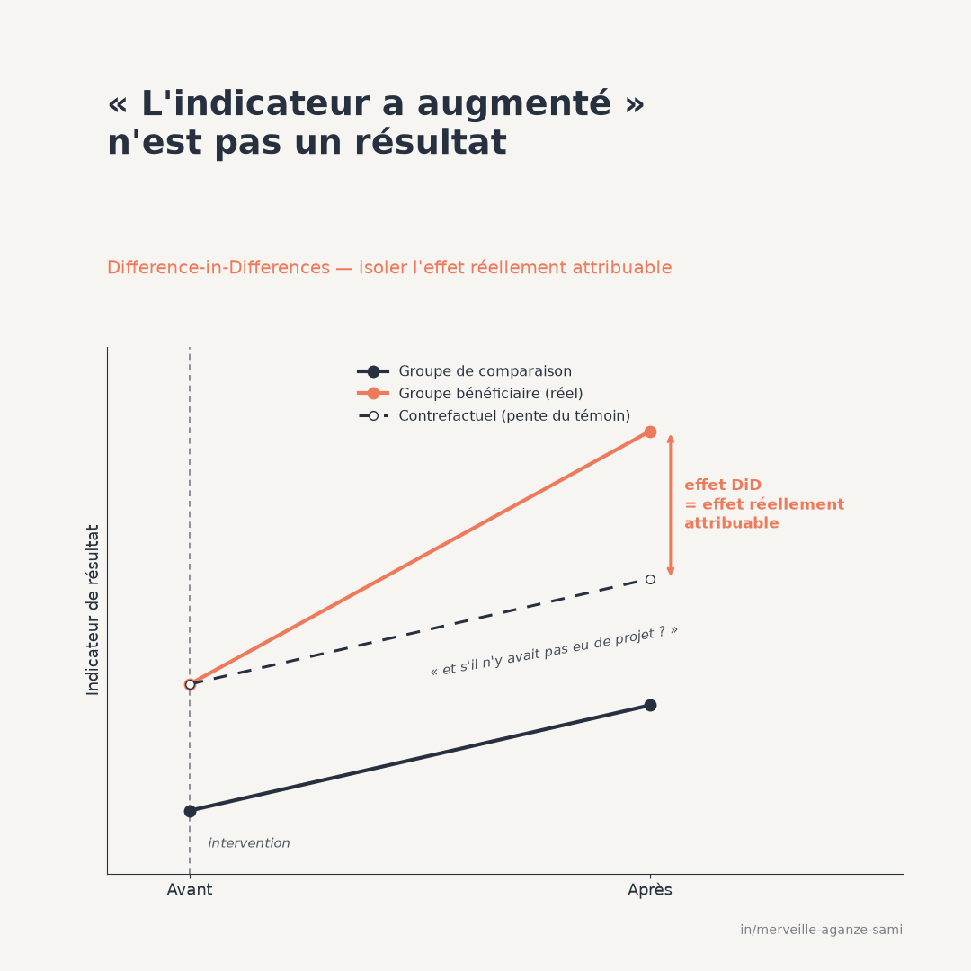
The most common reading of a project result compares an indicator before and after the intervention among beneficiaries. A rise is then interpreted as an effect. This inference implicitly assumes that, absent the project, the indicator would have remained stable.

That assumption is rarely warranted. A favourable agricultural season, a price movement, a national policy or a dynamic already under way before the first activity produce variations independent of the intervention. A before-after comparison on the beneficiary group alone aggregates the project effect and all of these factors.

1. What difference-in-differences isolates

The method follows two groups — beneficiaries and a comparison group — over at least two periods. It computes the change in the indicator within each group, then the difference between those two changes. The reasoning is explicit: whatever affected both groups in the same way cancels in the subtraction; what remains is attributable to what distinguishes the two groups, namely the intervention.

The classic illustration of this approach in public policy evaluation rests on comparing two territories subject to different rules, one serving as a reference for the other (Card & Krueger, 1994). The principle applies equally to a development project with partial geographic coverage.

2. The parallel trends assumption

The identifying condition reads: absent the intervention, the two groups would have experienced the same change. It does not assume they were identical — a constant level difference is allowed and cancels in the double difference — but that their trajectories would have been parallel.

This assumption concerns a situation that did not occur; it cannot therefore be demonstrated. It can, however, be made more or less plausible by examining pre-intervention periods: if the two groups followed parallel trajectories over several periods before the start, the assumption gains credibility.

3. Checking pre-trends without being reassured by them

Plotting period-by-period gaps, before and after the intervention, is the usual check. It calls for two reservations. First, a test on prior periods often lacks power: no detected gap does not mean no gap. Second, selecting cases on the basis of that test introduces bias into the estimates retained, a documented effect that invites treating this check as an element of judgement rather than a validation criterion (Roth, 2022).

The recommended approach is therefore to present the pre-period plot, to state the assumption as an assumption, and to examine the sensitivity of the result to plausible departures from parallelism.

4. Standard errors

A frequently underestimated difficulty concerns inference. Observations from the same geographic unit are correlated over time, and units within the same territory are correlated with one another. Treating observations as independent yields markedly understated standard errors and unfounded significance conclusions (Bertrand et al., 2004).

The usual correction clusters errors at the level at which treatment is assigned — territory, district, grouping. It nonetheless assumes a sufficient number of clusters; below about thirty, inference methods designed for few clusters are required. The number of clusters used should appear in the report, alongside the sample size (Angrist & Pischke, 2009).

5. When treatment starts at different dates

Many projects begin at different dates depending on the area. This configuration, long handled by a standard fixed-effects regression, raises a recently identified difficulty: the estimator implicitly combines comparisons between already-treated units and later-treated units, some of which receive negative weights when the effect varies over time (Goodman-Bacon, 2021).

Estimators designed for this case build explicit comparisons between cohorts entering at a given date and not-yet-treated units, then aggregate these effects under transparent weighting (Callaway & Sant'Anna, 2021). Where entry dates differ, their use should be the rule rather than the exception.

6. Further points to document

• Sample composition. If the units observed differ between the two periods, the double difference partly measures a compositional change. A panel of the same units is preferable; failing that, the comparability of samples must be established.
• Anticipation effects. Prior announcement of the project may alter behaviour before actual start-up, contaminating the reference period. The date to use is that of first plausible influence, not that of the first activity.
• Spillover to the comparison group. If benefits partly reach the comparison group — geographic proximity, trade, mobility — the estimated effect is understated. A minimum distance between treated and comparison areas limits this risk.
• Selection on a temporary dip. Where targeting picks units experiencing a passing difficulty, their spontaneous recovery will be counted as an effect. Examining several prior periods reveals this configuration.

The question underpinning an impact evaluation is not whether an indicator rose, but against what reference that rise is measured. Constructing and justifying that reference is the substance of the methodological work.

Merveille Aganze Sami

MEL & Database Management Advisor. 9+ years of experience in monitoring & evaluation, GIS and digitalization with international organizations (GIZ, Enabel) in DR Congo.

LinkedIn Contact me

References

- Angrist, J. D., & Pischke, J.-S. (2009). Mostly Harmless Econometrics: An Empiricist's Companion. Princeton: Princeton University Press.
- Bertrand, M., Duflo, E., & Mullainathan, S. (2004). How Much Should We Trust Differences-in-Differences Estimates? The Quarterly Journal of Economics, 119(1), 249–275. doi.org/10.1162/003355304772839588
- Callaway, B., & Sant'Anna, P. H. C. (2021). Difference-in-Differences with multiple time periods. Journal of Econometrics, 225(2), 200–230. doi.org/10.1016/j.jeconom.2020.12.001
- Card, D., & Krueger, A. B. (1994). Minimum Wages and Employment: A Case Study of the Fast-Food Industry in New Jersey and Pennsylvania. American Economic Review, 84(4), 772–793.
- Goodman-Bacon, A. (2021). Difference-in-differences with variation in treatment timing. Journal of Econometrics, 225(2), 254–277. doi.org/10.1016/j.jeconom.2021.03.014
- Roth, J. (2022). Pretest with Caution: Event-Study Estimates after Testing for Parallel Trends. American Economic Review: Insights, 4(3), 305–322. doi.org/10.1257/aeri.20210236