Hot spots:
a structural cluster or an isolated value?

Territorial prioritisation commonly relies on a unit-by-unit comparison: each area is measured against a threshold, classified above or below, and the list of struggling areas is drawn up. This procedure implicitly treats units as independent of one another.

That assumption raises an interpretation difficulty. An area with a low indicator whose neighbours show comparable values describes a different situation from an isolated area surrounded by high values. The first suggests a regional determinant — an access barrier, an agro-ecological context, a failing structural service; the second more likely reflects a local cause or sampling variability. The two call for distinct responses.

1. What the local statistic measures

The Getis-Ord statistic compares, for each unit, the sum of values observed in its neighbourhood — including the unit itself in the starred version — with the sum that would be expected if values were distributed without spatial structure. The gap is standardised into a z-score whose sign indicates a cluster of high or low values and whose magnitude indicates the degree of departure from the no-structure hypothesis (Getis & Ord, 1992). The distributional properties of this family of local statistics were subsequently clarified (Ord & Getis, 1995).

2. The neighbourhood matrix is the main decision

The result depends directly on the definition of neighbourhood adopted. Four options are in common use, and the choice should be justified by the nature of the phenomenon rather than by the software default.

• Contiguity. Two units are neighbours if they share a boundary. Suited to a regular administrative mesh, this criterion becomes problematic where units are of very unequal size.
• Distance threshold. All units within a given distance are neighbours. The threshold should correspond to a scale meaningful for the phenomenon — catchment reach, mobility radius.
• k nearest neighbours. Each unit has the same number of neighbours, which homogenises treatment where density varies strongly, at the cost of a varying effective distance.
• Continuous weighting. Influence decays with distance rather than vanishing at a threshold. More realistic for diffusive phenomena, this option requires setting the form of decay.

Good practice is to test the sensitivity of the result to this choice: if identified hot spots shift substantially from one definition to another, the conclusion is not robust and should be presented as such.

3. The multiple testing problem

A local statistic is computed for every unit in the territory. Across several hundred units, a number of significant results appear through the sheer multiplicity of tests. Retaining a conventional threshold without correction therefore identifies clusters that are not clusters.

Two difficulties compound here: the multiplicity of tests and their dependence, since neighbourhoods overlap. A false discovery rate correction (Benjamini & Hochberg, 1995) is better suited than a highly conservative correction, and its application to the specific case of local spatial association statistics has been documented (Caldas de Castro & Singer, 2006). An alternative is to establish the reference distribution by permutation rather than through a theoretical approximation.

4. What can distort the reading

• Zoning effect. The result depends on the level of aggregation and on how units are drawn. The same phenomenon analysed at health-zone or health-area level can produce different hot spot maps. This dependence is a general property of spatially aggregated data (Fotheringham & Wong, 1991).
• Counts versus rates. A statistic computed on counts largely reflects population distribution. The analysis must use a rate or proportion where the question concerns relative intensity.
• Unstable variance on small populations. A rate computed on a small denominator has high variability, producing extreme values unrelated to any real phenomenon. Prior smoothing or a method accounting for the denominator is then required.
• Confusing significance with magnitude. A significant value indicates a cluster that is improbable under the no-structure hypothesis, not a high level of need. Prioritisation must combine spatial significance with the level of the indicator.

5. Use for prioritisation

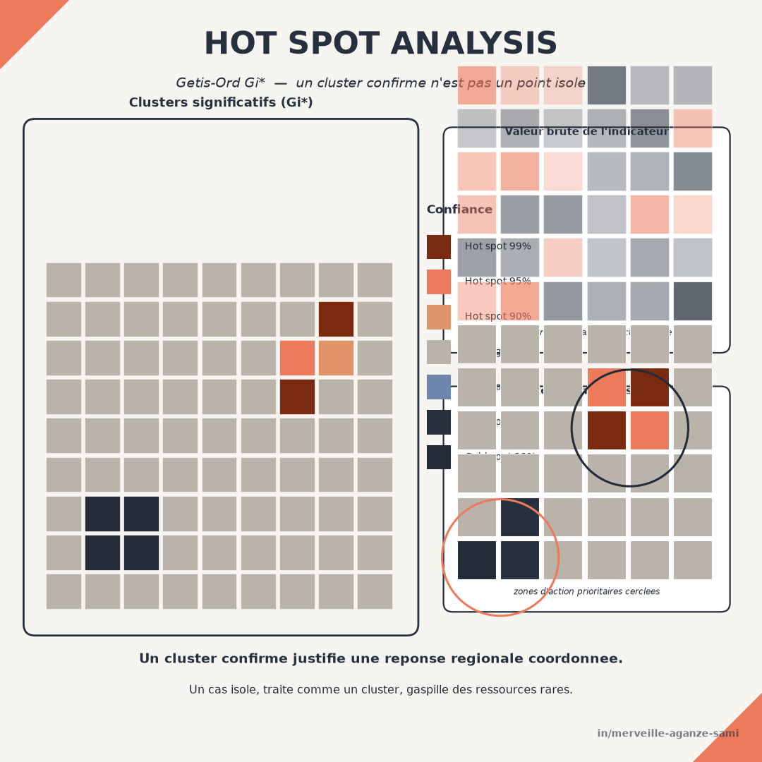
Combined with the raw indicator value, the local statistic yields a four-position reading grid: an unfavourable value within a significant cluster, justifying a coordinated response at group scale; an isolated unfavourable value, calling for local diagnosis; a favourable value within a cluster, which may serve as a reference; and an isolated favourable value, whose atypical character warrants examination.

This grid makes the targeting decision explainable. It indicates not only where to intervene but at what scale — a trade-off that usually remains implicit in a simple ranked list of areas.

Spatial significance does not replace the value of the indicator; it qualifies its scope. It indicates whether a local finding reflects a wider phenomenon or a particular situation, and that distinction determines the scale of the response.

Merveille Aganze Sami

MEL & Database Management Advisor. 9+ years of experience in monitoring & evaluation, GIS and digitalization with international organizations (GIZ, Enabel) in DR Congo.

LinkedIn Contact me

References

- Anselin, L. (1995). Local Indicators of Spatial Association—LISA. Geographical Analysis, 27(2), 93–115. doi.org/10.1111/j.1538-4632.1995.tb00338.x
- Benjamini, Y., & Hochberg, Y. (1995). Controlling the False Discovery Rate: A Practical and Powerful Approach to Multiple Testing. Journal of the Royal Statistical Society: Series B, 57(1), 289–300. doi.org/10.1111/j.2517-6161.1995.tb02031.x
- Caldas de Castro, M., & Singer, B. H. (2006). Controlling the False Discovery Rate: A New Application to Account for Multiple and Dependent Tests in Local Statistics of Spatial Association. Geographical Analysis, 38(2), 180–208. doi.org/10.1111/j.0016-7363.2006.00682.x
- Fotheringham, A. S., & Wong, D. W. S. (1991). The modifiable areal unit problem in multivariate statistical analysis. Environment and Planning A, 23(7), 1025–1044. doi.org/10.1068/a231025
- Getis, A., & Ord, J. K. (1992). The Analysis of Spatial Association by Use of Distance Statistics. Geographical Analysis, 24(3), 189–206. doi.org/10.1111/j.1538-4632.1992.tb00261.x
- Ord, J. K., & Getis, A. (1995). Local Spatial Autocorrelation Statistics: Distributional Issues and an Application. Geographical Analysis, 27(4), 286–306. doi.org/10.1111/j.1538-4632.1995.tb00912.x