Propensity score matching:
building a credible counterfactual

A common practice in evaluation is to compare a group of beneficiaries with a group of non-beneficiaries, then attribute the measured gap to the programme. This reading assumes the two groups were comparable before the intervention. That condition is rarely met in the field.

Participation in a project almost always results from a selection process: targeting through eligibility criteria, self-selection of the most available or best-informed households, proximity to an access road. The gap observed at the end of the programme therefore aggregates two components: the effect of the intervention and the pre-existing differences between the groups. This confounding constitutes selection bias, whose magnitude may exceed that of the effect being sought (Heckman et al., 1997).

1. The principle of the propensity score

The propensity score is defined as the probability, for a given unit, of receiving the treatment given its characteristics observed before the intervention. It is most often estimated by a logistic regression whose dependent variable is participation and whose explanatory variables are baseline characteristics: household size, education, productive assets, distance to a centre, initial value of the outcome of interest.

This property holds only under an explicit assumption, known as conditional independence: every variable that jointly influences participation and the outcome must appear in the model. It is an identifying assumption, not a result the data can demonstrate.

2. Five implementation steps

1. 1Specify the covariates. Retain only variables measured before the intervention or structurally invariant. Including a post-treatment variable, itself affected by the programme, introduces further bias.
2. 2Estimate the score. A logistic regression suffices in most cases. The aim is not to maximise the model's predictive performance but to obtain a score that balances the groups.
3. 3Choose the matching algorithm. Nearest neighbour with or without replacement, kernel matching, stratification, or inverse probability weighting. Each option trades bias against variance; the respective properties are documented (Caliendo & Kopeinig, 2008).
4. 4Impose common support and a caliper. Treated units whose score has no counterpart in the comparison group must be dropped or flagged. A maximum score distance — the caliper — prevents accommodating matches between distant profiles.
5. 5Check balance. Not an optional step: it is balance, not estimation, that validates the matching.

3. Diagnosing balance rather than fit

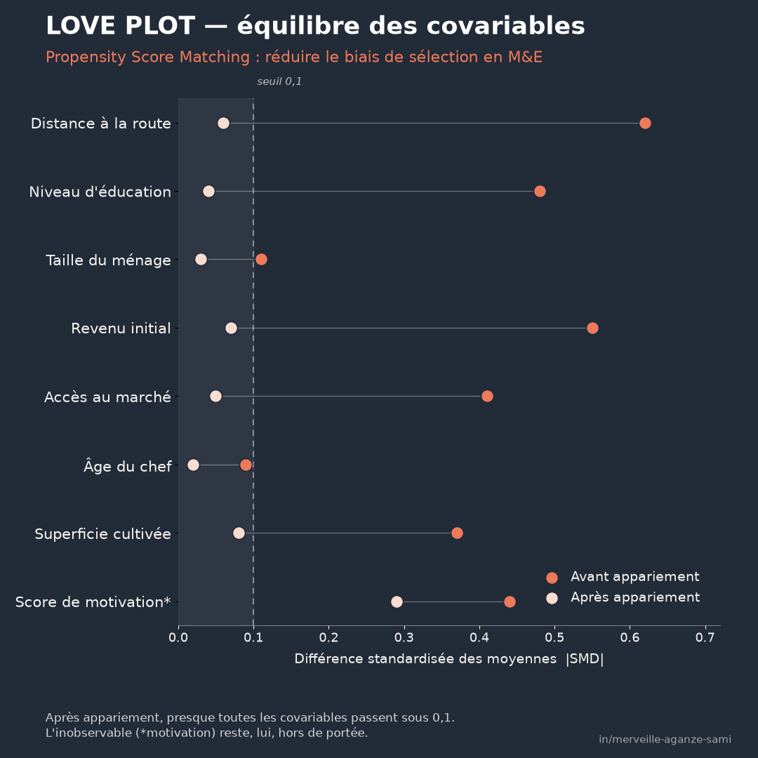
The quality of a matching procedure is not judged by the significance of the coefficients in the participation model, but by the effective reduction of differences between groups. The usual indicator is the standardised mean difference, computed covariate by covariate before and after matching.

The methodological literature conventionally treats an absolute value below 0.1 as indicating acceptable balance; this is a pragmatic benchmark rather than a statistical threshold (Austin, 2011). Plotting these differences before and after matching — often called a love plot — shows in a single figure whether the operation has genuinely tightened the distributions. Examining the overlap of score distributions and, for continuous variables, variance ratios is also recommended (Stuart, 2010).

4. Limitations to document

• The unobserved remains out of reach. Motivation, social capital and prior information do not appear in routine survey data. Matching leaves them intact. A sensitivity analysis, indicating how strong an unobserved factor would have had to be to overturn the result, at least quantifies the stake.
• Matching on the score is not always the best choice. Research has shown that matching based on the propensity score alone can, in certain configurations, degrade balance relative to methods matching directly on covariates. This critique concerns the use of the score for matching, not the propensity score family as a whole (King & Nielsen, 2019).
• Standard errors must account for matching. Treating the matched sample as an ordinary sample understates uncertainty, since the score is itself estimated. Resampling or appropriate variance estimators are required.
• Restricting to common support changes the population of inference. If a substantial share of treated units is dropped for lack of a counterpart, the estimated effect no longer applies to all beneficiaries. The matching rate must be reported.

5. Position within an evaluation design

Propensity score matching does not replace random assignment; it provides an approximation in the situations — the majority in development cooperation — where randomisation is neither feasible nor acceptable. Its credibility rests on the richness of baseline data: a well-designed baseline survey covering the plausible determinants of participation conditions validity far more than the sophistication of the chosen algorithm.

Where data are available before and after the intervention for both groups, combining matching with difference-in-differences markedly strengthens the argument: it neutralises time-invariant differences, including unobserved ones, that persist after matching.

The useful question upstream of an evaluation is not what gap separates the two groups, but how far those groups were comparable before the intervention. The answer determines what the measured gap allows one to conclude.

Merveille Aganze Sami

MEL & Database Management Advisor. 9+ years of experience in monitoring & evaluation, GIS and digitalization with international organizations (GIZ, Enabel) in DR Congo.

LinkedIn Contact me

References

- Austin, P. C. (2011). An Introduction to Propensity Score Methods for Reducing the Effects of Confounding in Observational Studies. Multivariate Behavioral Research, 46(3), 399–424. doi.org/10.1080/00273171.2011.568786
- Caliendo, M., & Kopeinig, S. (2008). Some Practical Guidance for the Implementation of Propensity Score Matching. Journal of Economic Surveys, 22(1), 31–72. doi.org/10.1111/j.1467-6419.2007.00527.x
- Heckman, J. J., Ichimura, H., & Todd, P. E. (1997). Matching as an Econometric Evaluation Estimator: Evidence from Evaluating a Job Training Programme. The Review of Economic Studies, 64(4), 605–654. doi.org/10.2307/2971733
- King, G., & Nielsen, R. (2019). Why Propensity Scores Should Not Be Used for Matching. Political Analysis, 27(4), 435–454. doi.org/10.1017/pan.2019.11
- Rosenbaum, P. R., & Rubin, D. B. (1983). The Central Role of the Propensity Score in Observational Studies for Causal Effects. Biometrika, 70(1), 41–55. doi.org/10.1093/biomet/70.1.41
- Stuart, E. A. (2010). Matching Methods for Causal Inference: A Review and a Look Forward. Statistical Science, 25(1), 1–21. doi.org/10.1214/09-STS313