Spatial autocorrelation:
signal or chance?

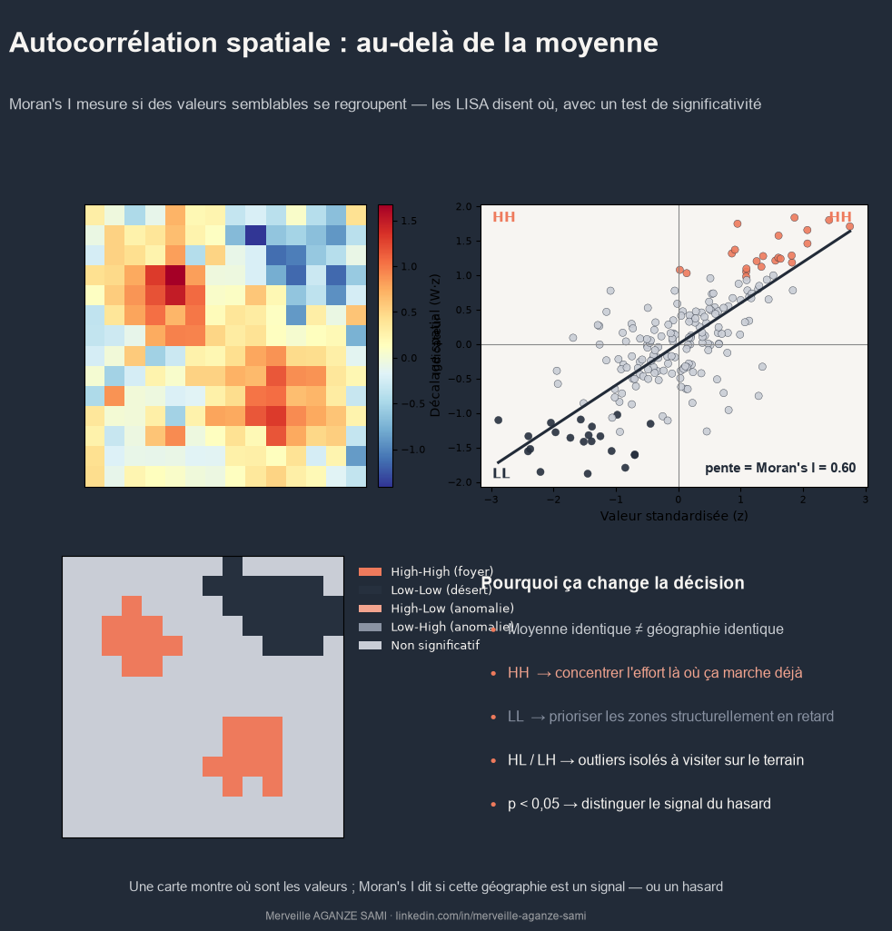
Two regions may exhibit exactly the same mean for a given indicator while describing two opposite geographical realities. In the first, high values are evenly distributed; in the second, they concentrate in two clusters surrounded by poorly endowed areas. Neither the mean nor a choropleth map distinguishes these configurations — yet the appropriate programmatic response differs.

Spatial autocorrelation analysis provides a statistical framework for this question. It rests on an intuition formalised by Waldo Tobler in 1970, whereby nearby entities tend to resemble one another more than distant ones (Tobler, 1970). The operational question then becomes measurable: is the observed clustering consistent with a random distribution, or does it reflect a structure?

1. The neighbourhood matrix: a prior methodological decision

Any autocorrelation statistic requires a prior definition of what "neighbour" means. This definition takes the form of a spatial weights matrix W, whose specification conditions all subsequent results. The most common conventions rest on contiguity — two units sharing an edge (rook criterion) or merely a vertex (queen criterion) — or on distance, by threshold or by a fixed number of nearest neighbours.

The matrix is generally row-standardised, so that the weights of each unit sum to one. This choice is not neutral: an overly broad neighbourhood definition dilutes local structures, while an overly restrictive one artificially isolates units. Documenting this choice is an integral part of reporting results (Anselin, 1995).

2. Global Moran's I: a summary measure

Proposed by Patrick Moran in 1950, the I statistic compares the covariance between each unit and its neighbours with the total variance of the variable (Moran, 1950). Its value is read on a scale ranging approximately from −1 to +1: a markedly positive value indicates that similar units are neighbours (clustering), a value close to zero a distribution consistent with chance, and a negative value a checkerboard configuration in which dissimilar units adjoin.

Significance is assessed by comparison with a reference distribution obtained through random permutations of values across geographical units. The resulting pseudo p-value indicates how frequently a structure at least as pronounced would arise under the hypothesis of spatial independence (Cliff & Ord, 1981).

3. LISA: locating the structures

Local indicators of spatial association, formalised by Luc Anselin, decompose the global index into individual contributions. Each unit receives its own local statistic and significance, allowing classification into one of the four quadrants of the Moran scatterplot (Anselin, 1995):

• High-High: a high-value unit surrounded by high-value units — a concentration cluster.
• Low-Low: a low-value unit surrounded by low-value units — a structurally lagging area.
• High-Low and Low-High: values atypical relative to their neighbourhood — spatial outliers warranting field verification.
• Non-significant: a configuration consistent with a random distribution.

The Getis-Ord Gi* statistic pursues a related objective through a different logic: it compares the sum of values within a neighbourhood with the sum expected under independence, and explicitly distinguishes clusters of high values from clusters of low values (Getis & Ord, 1992). LISA and Gi* are not interchangeable: the former also identifies isolated outliers, the latter lends itself better to hot-spot and cold-spot mapping.

4. Interpretation caveats

Three caveats condition the validity of conclusions.

• Multiple comparisons. Simultaneously testing several hundred units multiplies false positives. A correction, for instance the Benjamini-Hochberg procedure, is recommended before interpreting significance maps.
• Effect of the spatial support. Results depend on the administrative zoning used. This phenomenon, known as the modifiable areal unit problem, means that the same data aggregated differently may yield divergent conclusions.
• Edge effects. Units on the periphery of the study area mechanically have fewer neighbours, which biases their local statistic.

5. Operational significance

For a monitoring and evaluation system, the contribution is direct. Identifying High-High clusters allows resources to be concentrated where momentum already exists; identifying Low-Low areas signals territories whose lag is structural rather than circumstantial. Isolated outliers, for their part, are natural candidates for a verification mission, insofar as they suggest a local factor not captured by available data.

The analysis thus turns a descriptive map into a documented targeting instrument. Above all, it provides a defensible argument: prioritisation no longer rests on visual reading of a map, but on a statistical test whose method, parameters and threshold can be made explicit.

Merveille Aganze Sami

MEL & Database Management Advisor. 9+ years of experience in monitoring & evaluation, GIS and digitalization with international organizations (GIZ, Enabel) in DR Congo.

LinkedIn Contact me

References

- Anselin, L. (1995). Local Indicators of Spatial Association—LISA. Geographical Analysis, 27(2), 93–115. doi.org/10.1111/j.1538-4632.1995.tb00338.x
- Cliff, A. D., & Ord, J. K. (1981). Spatial Processes: Models and Applications. London: Pion.
- Getis, A., & Ord, J. K. (1992). The Analysis of Spatial Association by Use of Distance Statistics. Geographical Analysis, 24(3), 189–206. doi.org/10.1111/j.1538-4632.1992.tb00261.x
- Moran, P. A. P. (1950). Notes on Continuous Stochastic Phenomena. Biometrika, 37(1/2), 17–23. doi.org/10.2307/2332142
- Tobler, W. R. (1970). A Computer Movie Simulating Urban Growth in the Detroit Region. Economic Geography, 46, 234–240. doi.org/10.2307/143141