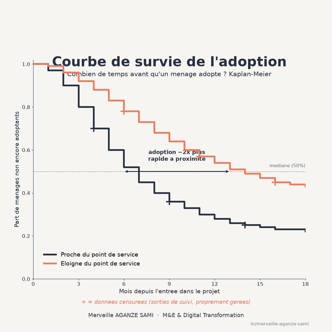
Monitoring systems generally report adoption of a practice through a rate measured at the end of the period: the proportion of households that adopted. This measure has the drawback of being a state, whereas the phenomenon studied is a process unfolding over time.
Two projects reporting the same final rate may cover opposite dynamics: in one, most adoptions occurred within the first three months; in the other, they spread over two years. These two situations call for neither the same diagnosis nor the same operational decision.
1. The problem with computing a rate
A technical difficulty compounds this loss of information. Not all households are observed for the same length of time: some join partway through, others leave — relocation, withdrawal, end of the observation period. At the time of computation, all that is known is that they had not adopted up to that point.
Right censoring. These partial observations are neither adoptions nor non-adoptions: they constitute information about a minimum duration. Excluding them removes valid data and biases the result; counting them as non-adoptions asserts information one does not have. Survival analysis methods are built precisely to exploit this partial information.
2. Estimating the adoption curve
The reference non-parametric estimator reconstructs the probability of not yet having adopted at each point in time, updating that probability at each observed event and removing censored units from the denominator (Kaplan & Meier, 1958). The result is a step curve whose reading directly yields operational quantities.
The most useful is median time — the duration by which half the households have adopted. A mean is generally not computable under censoring, since the duration remains unknown for part of the sample. Comparison between two groups uses a dedicated test comparing the whole curves rather than a single point (Bland & Altman, 2004).
3. Quantifying the effect of factors
The proportional hazards model estimates the effect of several characteristics on the pace of adoption — distance to the service point, household composition, type of support — without imposing a particular form on the baseline curve (Cox, 1972). Each coefficient is interpreted as an instantaneous rate ratio: a value of 1.5 indicates a pace of adoption half again as fast, at comparable other characteristics.
One interpretive point matters here. The model describes a conditional association, not a causal effect. Attributing a causal role to a factor requires a separate identification design, such as the one presented in the article on propensity score matching.
4. Checking the model's assumption
The model assumes the rate ratio between two profiles stays constant over time. This assumption can be checked by examining residuals, and it is frequently violated in practice: close-support arrangements may sharply accelerate adoption in the early months and then cease to differentiate (Grambsch & Therneau, 1994).
Where the assumption does not hold, two responses exist: stratify the model on the variable concerned, or introduce an interaction with time. Flagging the violation without addressing it yields coefficients whose interpretation is not the one announced.
5. Points to handle in a field system
- Definition of the event. “Adopting” must correspond to an observable, dated criterion. A vague definition produces a duration variable whose measurement varies by enumerator.
- Interval censoring. Where monitoring visits are periodic, all that is known is that adoption occurred between two visits. Treating the visit date as the event date introduces systematic bias; methods for interval-censored data exist and should be used where visits are widely spaced.
- Informative censoring. If the households that leave monitoring are precisely those that would not have adopted, the estimate is optimistically biased. Reasons for exit must be recorded and analysed.
- Competing risks. A household that leaves the area or abandons the activity is not in the same situation as one still liable to adopt. Treating such exits as plain censoring overstates the probability of adoption; estimators accounting for competing events correct this bias (Fine & Gray, 1999).
- Within-village correlation. Households in the same locality share unobserved determinants. Standard errors must account for this, failing which precision is overstated.
6. Integration into the collection tool
The practical condition is simple but often missing: the collection form must record event dates, not a binary status at the visit date. This modification, minor in tooling terms, conditions the entire analysis. Each timestamped visit then feeds a curve that updates as data arrive (Clark et al., 2003).
The dashboard thereby moves from a state indicator — is the target met — to a pace indicator, which flags a slowdown before the final rate is compromised.
Key points
- A final rate aggregates two very different dynamics: fast then flat, or slow and steady
- Exits from monitoring are minimum-duration information, not non-adoptions
- Median time is the readable quantity; the mean is generally not computable
- The proportional hazards model describes an association, not a causal effect
- The form must record event dates, not a status at the visit date
In programme monitoring, the question of “how many” frequently conceals a more directly actionable question of “when”. Measuring pace allows intervention mid-process; measuring a state only allows reporting after the fact.
References
- Bland, J. M., & Altman, D. G. (2004). The logrank test. BMJ, 328(7447), 1073. doi.org/10.1136/bmj.328.7447.1073
- Clark, T. G., Bradburn, M. J., Love, S. B., & Altman, D. G. (2003). Survival Analysis Part I: Basic concepts and first analyses. British Journal of Cancer, 89(2), 232–238. doi.org/10.1038/sj.bjc.6601118
- Cox, D. R. (1972). Regression Models and Life-Tables. Journal of the Royal Statistical Society: Series B, 34(2), 187–202. doi.org/10.1111/j.2517-6161.1972.tb00899.x
- Fine, J. P., & Gray, R. J. (1999). A Proportional Hazards Model for the Subdistribution of a Competing Risk. Journal of the American Statistical Association, 94(446), 496–509. doi.org/10.1080/01621459.1999.10474144
- Grambsch, P. M., & Therneau, T. M. (1994). Proportional hazards tests and diagnostics based on weighted residuals. Biometrika, 81(3), 515–526. doi.org/10.1093/biomet/81.3.515
- Kaplan, E. L., & Meier, P. (1958). Nonparametric Estimation from Incomplete Observations. Journal of the American Statistical Association, 53(282), 457–481. doi.org/10.1080/01621459.1958.10501452

Merveille Aganze Sami
MEL & Database Management Advisor. 9+ years of experience in monitoring & evaluation, GIS and digitalization with international organizations (GIZ, Enabel) in DR Congo.
Adoption monitoring to structure?
Get in touch