Surface water:
why the reference index fails in cities

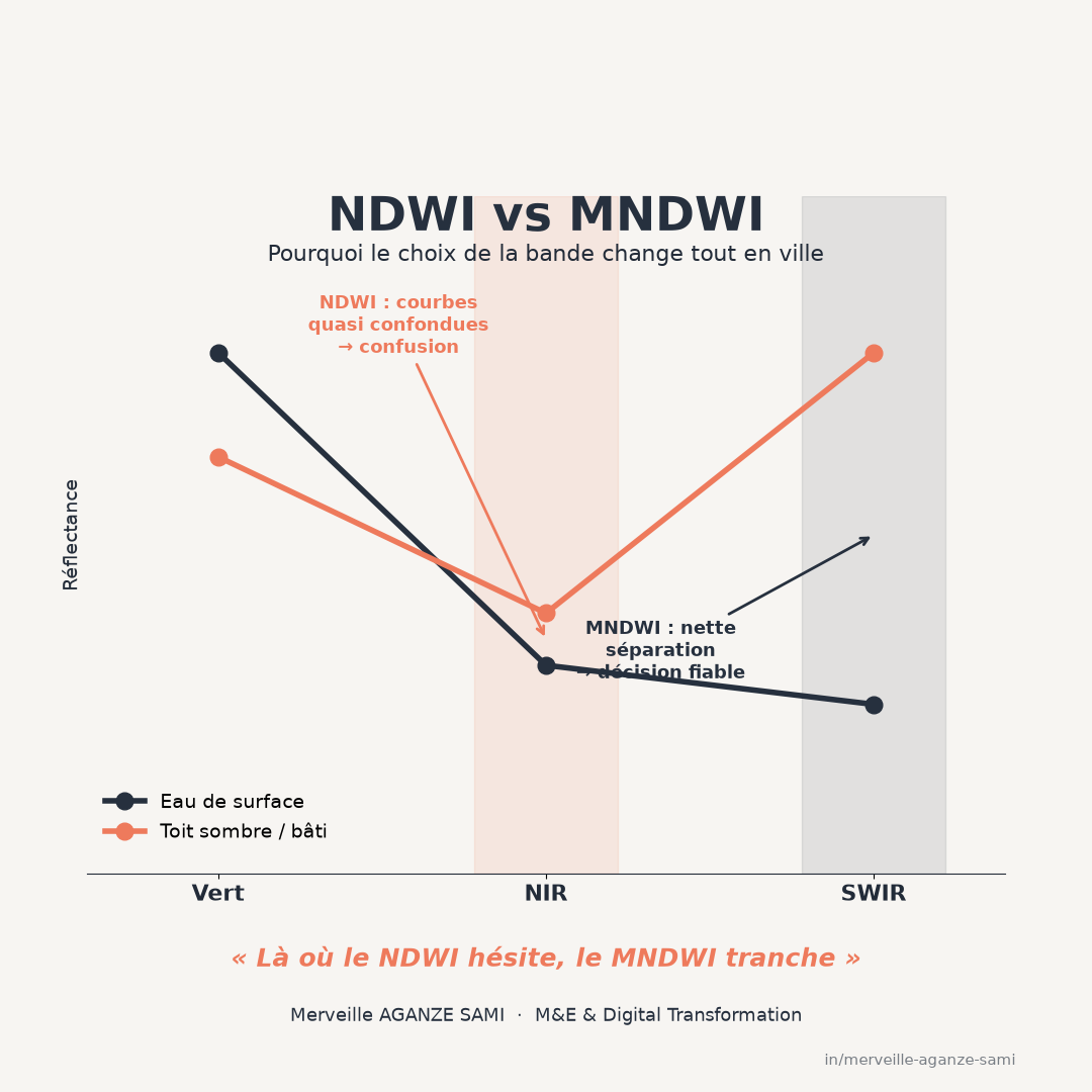
Delineating surface water from satellite imagery commonly relies on a normalised index combining the green and near infrared bands. This formulation exploits a clear physical property: water absorbs strongly in the near infrared whereas vegetation and soils reflect there (McFeeters, 1996).

The resulting contrast is excellent over an isolated water body, an open river or a flooded area in a rural setting. It degrades markedly, however, in dense urban settings, where the index classifies as water surfaces that are not: dark roofs, wet asphalt, building shadows.

1. Where the problem originates

The confusion stems from the band used. In the near infrared, water and many dark artificial surfaces have similar reflectance. The normalised ratio opposing them to the green band then produces close values, and no threshold separates them reliably.

This ambiguity has an immediate operational consequence: it concentrates precisely in inhabited areas, that is, where a flood map drives alert or assistance decisions. Over-detection there is therefore particularly problematic.

2. Substituting the band

On Sentinel-2 this formulation uses bands B3 and B11; on Landsat 8/9, bands 3 and 6. A difference in native resolution between the two bands must be handled by resampling, an operation whose method deserves documenting since it affects the sharpness of the resulting boundaries.

3. Multi-band formulations

Where a scene contains both dark built surfaces and pronounced shadow — terrain, tall buildings — two bands do not always suffice. Indices combining four to five bands have been developed to improve separation in such configurations, with variants depending on whether the scene contains extensive artificial surfaces (Feyisa et al., 2014).

Systematic comparisons between methods show that no formulation dominates in all contexts, and that performance depends on landscape type, water turbidity and the presence of aquatic vegetation (Fisher et al., 2016). The choice is therefore a matter of local testing, not of principle.

4. The threshold question

An index produces a continuous value; the water map results from thresholding. A value of zero is frequently used by default, but it has no universal basis: the optimal value depends on turbidity, depth, submerged vegetation and illumination conditions.

• Adaptive thresholding. Deriving the threshold from each image's histogram, rather than fixing it once and for all, improves stability between dates.
• Validation on reference points. A few dozen water and non-water points, identified on high-resolution imagery, allow omission and commission rates to be estimated and the threshold calibrated.
• Permanent water mask. Distinguishing permanent from seasonal water requires a multi-year reference; global datasets provide this baseline and allow the event component to be isolated (Pekel et al., 2016).
• Temporal consistency. For seasonal monitoring, threshold and method must remain identical across dates, failing which the measured change partly reflects a change in processing.

5. Limits of the optical approach

• Cloud cover. Flood events frequently coincide with weather unfavourable to optical observation. A usable image may only become available several days after the peak, which limits use in emergency response. Radar imagery, insensitive to clouds, addresses this constraint — a topic developed in the article on radar flood mapping.
• Water under vegetation. An area flooded beneath a dense canopy is not detected: the signal comes from the vegetation, not the water beneath.
• Shallow, turbid water. A thin sediment-laden water layer has a signature intermediate between water and bare soil, producing omissions in flood zones.
• Mixed pixels. At ten or twenty metre resolution, water body edges and narrow watercourses occupy a fraction of a pixel. The estimated area then depends strongly on the threshold adopted.

No spectral index is optimal independently of the landscape observed. The useful reflex is not to adopt the most-cited formulation, but to check which one actually separates the categories that matter in the context studied.

Merveille Aganze Sami

MEL & Database Management Advisor. 9+ years of experience in monitoring & evaluation, GIS and digitalization with international organizations (GIZ, Enabel) in DR Congo.

LinkedIn Contact me

References

- Feyisa, G. L., Meilby, H., Fensholt, R., & Proud, S. R. (2014). Automated Water Extraction Index: A new technique for surface water mapping using Landsat imagery. Remote Sensing of Environment, 140, 23–35. doi.org/10.1016/j.rse.2013.08.029
- Fisher, A., Flood, N., & Danaher, T. (2016). Comparing Landsat water index methods for automated water classification in eastern Australia. Remote Sensing of Environment, 175, 167–182. doi.org/10.1016/j.rse.2015.12.055
- McFeeters, S. K. (1996). The use of the Normalized Difference Water Index (NDWI) in the delineation of open water features. International Journal of Remote Sensing, 17(7), 1425–1432. doi.org/10.1080/01431169608948714
- Pekel, J.-F., Cottam, A., Gorelick, N., & Belward, A. S. (2016). High-resolution mapping of global surface water and its long-term changes. Nature, 540, 418–422. doi.org/10.1038/nature20584
- Xu, H. (2006). Modification of normalised difference water index (NDWI) to enhance open water features in remotely sensed imagery. International Journal of Remote Sensing, 27(14), 3025–3033. doi.org/10.1080/01431160600589179